Kubernetes

 

Kubernetes is a Container Orchestration tool.

Multiple containers do run in worket nodes.

Features:

• High Availability
• Scalability
• Disaster Recovery

Basic Architecture:

It's basic Architecture contains Pods & Containers

1 Pod per Application, each pod contains 1 or more containers

Typically, 1 pod contains 1 container, however in cases when an application needs to access more than 1 resource like Database is in 1 container, messaging system is in another Container etc.

Why Spark on Kubernetes?

1. Multiple kinds of applications can run with each having it's own library dependency in the form of containers. 

Eg: In a cluster the below different kinds of applications can run simultaneously having their own library dependency.

•      Spark Applications can run in their own container.
•      ML Applications can run in a separate container. ML Libraries need not be installed in the cluster.

2. Spark cluster is a shared resource and if an upgrade needs to happen from Spark 2.0 to Spark 3.0 all the applications needs to be migrated. Incase of Kubernetes, only the applications those need to be upgraded can upgrade their dependencies and can run in their independent containers.

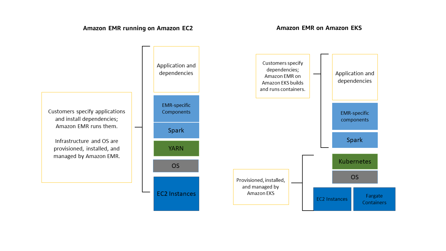
AWS EKS

The following diagram shows the two different deployment models for Amazon EMR.

Job Submission Options:

1. AWS Command line Interface
2. AWS Tools and AWS SDK
3. Apache Airflow

Sample command to Launch a PySpark job on AWS EMR on EKS

aws emr-containers start-job-run \

    --virtual-cluster-id <EMR-EKS-virtual-cluster-id> \

    --name <your-job-name> \

    --execution-role-arn <your-emr-on-eks-execution-role-arn> \

    --release-label emr-6.x.x \

    --job-driver '{

        "sparkSubmitJobDriver": {

            "entryPoint": "s3://<your-s3-bucket>/scripts/your_pyspark_script.py",

            "entryPointArguments": ["arg1", "arg2"],

            "sparkSubmitParameters": "--conf spark.executor.instances=2 --conf spark.executor.memory=2G --conf spark.driver.memory=1G"

        }

    }' \

    --configuration-overrides '{

        "applicationConfiguration": [

            {

                "classification": "spark-defaults",

                "properties": {

                    "spark.hadoop.fs.s3a.impl": "org.apache.hadoop.fs.s3a.S3AFileSystem",

                    "spark.kubernetes.container.image": "<your-custom-emr-on-eks-image-uri>"

                }

            }

        ],

        "monitoringConfiguration": {

            "s3MonitoringConfiguration": {

                "logUri": "s3://<your-s3-bucket>/logs/"

            },

            "cloudWatchMonitoringConfiguration": {

                "logGroupName": "<your-cloudwatch-log-group-name>",

                "logStreamPrefix": "<your-log-stream-prefix>"

            }

        }

    }'

--virtual-cluster-id: The ID of the virtual cluster registered with your EKS

Reference: https://www.youtube.com/watch?v=avXbYBPzpIE&t=649s

AWS Glue vs Running Spark jobs on EMR using spark-submit

 

comparison of AWS Glue vs Running Spark jobs on EMR using spark-submit vs AWS Sagemaker from a data engineering perspective:

---

1️⃣ AWS Glue

• Type: Serverless ETL service (managed Spark)

• When to Use: Lightweight to medium ETL/ELT workloads, event-driven or scheduled jobs.

• Pros:

  • Fully managed, no cluster management.

  • Auto-scaling and pay-per-use.

  • Built-in crawler, schema inference, and Data Catalog integration.

  • Native connectors to S3, RDS, Redshift, DynamoDB.

• Cons:

  • Limited cluster customization.

  • Startup latency (1–2 min warmup).

  • Less control over Spark version tuning.

Example:
ETL pipelines that transform S3 data to Redshift or Iceberg tables on S3.

---

2️⃣ Amazon EMR with spark-submit

• Type: Managed Hadoop/Spark cluster service (full control).

• When to Use: Heavy processing, streaming jobs, or when you need fine-grained control.

• Pros:

  • Full control over cluster configuration (memory, cores, Spark version).

  • Supports complex, long-running, streaming, and ML pipelines.

  • Can integrate with S3 (EMRFS), HDFS, Iceberg, Delta Lake.

• Cons:

  • You manage cluster lifecycle (start/stop or auto-terminate).

  • Higher ops overhead and cost if not managed well.

Example:
Petabyte-scale ETL, Spark Streaming with Kafka, or ML pipelines needing custom Spark configs.

---

💡 Rule of Thumb:

• Glue → Simpler, serverless ETL on S3/Redshift/Iceberg.

• EMR → Complex, large-scale, or streaming workloads needing control and custom tuning.

AWS Sagemaker

What is the difference between databricks and SageMaker?

SageMaker focuses on end-to-end ML workflows within the AWS ecosystem, offering tools for model training, deployment, and monitoring. In contrast, Databricks specializes in big data analytics and Spark-based ML, with strong collaboration features

Source: https://www.youtube.com/watch?v=95332cm5ROo

sagemaker schedule notebook vs processing job

Comparison of scheduled notebooks and processing jobs

Comparison of scheduled notebook vs. processing job

Feature	Scheduled Notebook Job	Processing Job
Primary Use Case	Moving an interactive Jupyter notebook into an automated, non-interactive execution for tasks like generating regular reports or running batch inferences.	Running production-level data processing and feature engineering scripts at scale.
Workflow	Streamlines the transition from an interactive environment to production. Data scientists can schedule their notebook directly from SageMaker Studio without converting code to a Python script.	Follows standard software development best practices. Requires moving code into a Python script and bundling dependencies, often using a custom container.
Reproducibility	A snapshot of the entire notebook is taken and executed. The output notebook with populated cells is saved, making it easy to review the results.	Highly reproducible because it runs a defined script within a controlled container environment. Inputs and outputs are strictly defined, typically to and from Amazon S3.
Containerization	SageMaker automatically handles packaging the notebook and its dependencies into a container. You can also specify an environment or startup script.	You must provide the script and dependencies, which are then run within a SageMaker-provided or custom Docker container.
Parameterization	Supports parameterization by using tags on notebook cells, allowing you to run the same notebook with different inputs for each execution.	Parameters are passed to the Python script at runtime, which is standard practice for scripting.
Scheduling Method	Scheduled directly from the SageMaker Studio UI or programmatically via the SageMaker Python SDK, which creates an EventBridge rule.	Can be scheduled through EventBridge, Lambda, or as a step within a SageMaker Pipeline.
Integration	Can be included as a step in a SageMaker Pipeline to create multi-step ML workflows.	Built for pipeline integration and is a fundamental component of SageMaker Pipelines.
Cost	You are charged for the duration of the job's execution on an ephemeral instance.	You are charged for the compute resources used during the job's execution, which are deprovisioned once the job is complete.

Step 1: Write your PySpark processing script

First, you need a Python script containing your PySpark logic. This script will be executed by the processing job.

• The script reads data from an S3 location provided as an argument.
• It performs a simple transformation (e.g., adding a new column).
• It writes the transformed data to a different S3 location. 

python

import argparse
import os
from pyspark.sql import SparkSession

if __name__ == '__main__':
    parser = argparse.ArgumentParser()
    parser.add_argument('--s3_input_path', type=str, required=True)
    parser.add_argument('--s3_output_path', type=str, required=True)
    args = parser.parse_args()

    # Initialize Spark Session
    spark = SparkSession.builder.appName("PySparkProcessingJob").getOrCreate()

    # Read data from S3
    df = spark.read.csv(args.s3_input_path, header=True, inferSchema=True)

    # Perform a simple transformation
    df_transformed = df.withColumn("new_feature", df["sepal_length"] * df["petal_length"])
    
    # Write the transformed data to S3
    df_transformed.write.parquet(args.s3_output_path, mode="overwrite")
    
    print("PySpark processing job finished.")

    spark.stop()

Step 2: Create and run the processing job with the SageMaker Python SDK

This Python code, which you can run in a SageMaker Studio notebook or any environment with the SageMaker SDK, performs the following:

1. Sets up a SageMaker session and gets your AWS role.
2. Uploads your PySpark script to an S3 bucket.
3. Creates a PySparkProcessor instance, specifying the desired Spark version and instance types for the cluster.
4. Defines the S3 locations for input data and output data.
5. Calls the run() method on the processor to start the job, passing the script and arguments. 

python

import sagemaker
from sagemaker.spark.processing import PySparkProcessor
from sagemaker.processing import ProcessingInput, ProcessingOutput
import boto3

# Setup your SageMaker session and role
sagemaker_session = sagemaker.Session()
role = sagemaker.get_execution_role()
region = boto3.Session().region_name

# Define the S3 bucket for data and script
bucket = sagemaker_session.default_bucket()
prefix = 'sagemaker-spark-processing'

# Upload the PySpark script to S3
script_path = sagemaker_session.upload_data(
    path='preprocess.py',
    bucket=bucket,
    key_prefix=f'{prefix}/code'
)

# Upload sample data to S3 for processing (for a real scenario, this would be your actual dataset)
sample_data_uri = f's3://sagemaker-sample-files/datasets/tabular/iris/iris.csv'

# Define the PySpark processor
spark_processor = PySparkProcessor(
    base_job_name="sm-pyspark-processing", # Recommended prefix for your jobs
    framework_version="3.1", # Specify your desired Spark version
    role=role,
    instance_count=2,
    instance_type="ml.m5.xlarge", # Use an instance type suitable for Spark
    sagemaker_session=sagemaker_session
)

# Define input and output paths
input_data_path = f'{sample_data_uri}'
output_data_path = f's3://{bucket}/{prefix}/output'

# Run the processing job
spark_processor.run(
    submit_app=script_path,
    inputs=[
        # For PySpark, you can reference the S3 path directly in the script
        # Alternatively, use ProcessingInput for automatic data copying
        # ProcessingInput(
        #     source=input_data_path,
        #     destination='/opt/ml/processing/input/data'
        # )
    ],
    outputs=[
        ProcessingOutput(
            source="/opt/ml/processing/output", # Directory on the instance where your script writes output
            destination=output_data_path,
            output_name="transformed_data"
        )
    ],
    arguments=[
        "--s3_input_path", input_data_path,
        "--s3_output_path", "/opt/ml/processing/output"
    ]
)

print(f"Processing job launched. Output will be in: {output_data_path}")

Delta Lake

Delta Lake is an open-source storage layer that brings ACID transactions, scalable metadata handling, and unified batch + streaming processing to big data workloads on top of Apache Spark and cloud object storage (like Azure Data Lake Storage, AWS S3, or GCS).

✅ Key Features of Delta Lake

Feature	Description
ACID Transactions	Guarantees data consistency through commits and rollbacks.
Schema Evolution	Automatically handles changes in data schema during writes.
Time Travel	Query older versions of data using versioning.
Unified Batch + Streaming	Use the same Delta table for both batch and real-time data processing.
Scalable Metadata	Supports billions of files and petabytes of data efficiently.
Data Reliability	Enforces schema, prevents partial or dirty writes.

🏗️ Delta Architecture: Bronze, Silver, Gold

1. Bronze Layer: Raw ingestion (streaming or batch from sources like Kafka, Event Hubs)

2. Silver Layer: Cleaned and transformed data

3. Gold Layer: Aggregated and business-ready data (used in dashboards)

Bronze Layer (Raw / Ingest)

Goal: Immutable as-received capture of source data with minimal transformation. Establish lineage and replayability.

Characteristics

• Schema: Often semi-structured (JSON, CSV, Avro) stored as ingested; may include _ingest_ts, _source_file, _source_system.

• Data Quality: Not validated beyond basic ingestion success.

• Storage Pattern: Partition by ingest date/time (e.g., ingest_date=YYYY-MM-DD) to simplify retention & replay.

• Use Cases: Reprocessing, audit, debugging, forensic analysis, schema drift detection.

• Append-only writes from streaming (readStream from Event Hubs/Kafka; Auto Loader for files).

Silver Layer (Clean / Conform / Enrich)

Goal: Turn raw data into analytics-grade canonical entities that are trustworthy and joinable across domains.

Transforms Typically Applied

Step	Examples
Data Cleansing	Drop corrupt rows; parse JSON; enforce data types.
Deduplication	Use event IDs, hashes, or window-based dedupe.
Normalization	Explode arrays; flatten nested structures.
Conformance	Standardize units, currencies, time zones (UTC), enums.
Joins / Enrichment	Lookup dimension tables (users, products, geo).
Watermark + Late Data Handling	Structured Streaming with withWatermark to discard/mark very late events.

Table Modeling

• Often entity-level (e.g., silver.sales_orders, silver.user_profile).

• Partition on business date (event_date, transaction_date) when high volume.

• Use MERGE INTO for CDC updates (upsert SCD Type 1/2 patterns).

Gold Layer (Curated / Business & Analytics)

Goal: High-trust, consumption-optimized data products: aggregates, KPIs, dimensional models, ML feature tables.

Patterns

Consumption Style	Modeling Approach	Notes
BI Reporting	Star/Snowflake (Fact + Dim tables)	Fast ad hoc BI (Power BI / Synapse).
Metrics/KPIs	Pre-aggregated summary tables	Daily/Hourly rollups, incremental refresh.
ML Features	Feature store–style Delta tables	Point-in-time correctness; training vs inference views.
Data Sharing	Cleaned, governed shareable tables	Unity Catalog + Delta Sharing.

Example Incremental ETL Flow (PySpark)

The Delta table is physically stored in your ADLS Gen2 container, mounted under /mnt/datalake/




# Bronze -> Silver incremental clean

bronze_path = "/mnt/datalake/bronze/events"

silver_table = "refined.silver.events_clean"

bronze_stream = (

  spark.readStream

       .format("delta")

       .load(bronze_path)

)

cleaned = (

  bronze_stream

    .filter("body IS NOT NULL")

    .selectExpr("cast(body as string) as json_str", "ingest_ts")

    .select(from_json("json_str", event_schema).alias("e"), "ingest_ts")

    .select("e.*", "ingest_ts")

    .dropDuplicates(["eventId"])

)

(cleaned.writeStream

    .format("delta")

    .outputMode("append")

    .option("checkpointLocation", "/mnt/datalake/checkpoints/silver/events_clean")

    .toTable(silver_table))

Silver → Gold Aggregation (Triggered Batch Refresh)

gold_table = "curated.gold.daily_event_metrics"

silver_df = spark.table("refined.silver.events_clean")

daily = (
  silver_df
    .groupBy("event_date", "channel")
    .agg(count("*").alias("event_count"),
         countDistinct("userId").alias("unique_users"))
)

(daily.write
      .format("delta")
      .mode("overwrite")
      .option("overwriteSchema", "true")
      .saveAsTable(gold_table))

Apache Iceberg

Apache Iceberg is a Lakehouse system with it's key as Metadata.

1. Storage

2. Processing

3. Metadata

        Metadata of Metadata

Key Points:

1. Storage

   • Data files (Parquet, ORC, Avro) are stored in Amazon S3.

   • Iceberg maintains metadata and snapshots to track table versions.

2. ACID Transactions

   • Supports atomic inserts, updates, and deletes directly on S3 data.

   • Prevents read/write conflicts in concurrent jobs.

3. Schema Evolution & Partitioning

   • Allows adding, dropping, or renaming columns without rewriting entire tables.

   • Supports hidden partitioning for efficient queries.

4. Query Engine Compatibility

   • Works with Spark, Flink, Trino, Presto, Athena, and Glue.

   • Enables time travel to query historical snapshots of data.

5. Lakehouse Advantage

   • Combines data lake storage (S3) with data warehouse-like capabilities.

   • Efficient for batch analytics, streaming, and ML pipelines.

---

🔹 Example Workflow on AWS:

1. Store raw/processed Parquet files in S3.

2. Create an Iceberg table referencing the S3 location.

3. Query and update data using Spark SQL or Athena with ACID guarantees.

4. Enable time travel for auditing or rollback.

Create Iceberg Table in Athena:

    CREATE TABLE iceberg_users (

        id INT,

        name STRING,

        event_date DATE

    )

    PARTITIONED BY = (day(event_date))

    LOCATION 's3://your-s3-bucket/iceberg-warehouse/iceberg_users/'

    TBLPROPERTIES (

        'table_type' = 'ICEBERG',

        'write.format.default' = 'parquet'

    );

Reference: https://www.youtube.com/watch?v=iGvj1gjbwl0

🔹 Operations using PySpark:

 Writing Data to an Iceberg Table

• Data files are stored as Parquet in S3.

• Metadata and snapshots are tracked by Iceberg in Glue catalog.

from pyspark.sql import SparkSession

# Initialize SparkSession with Iceberg support

spark = SparkSession.builder \

    .appName("IcebergReadWrite") \

    .config("spark.sql.catalog.glue_catalog", "org.apache.iceberg.spark.SparkCatalog") \

    .config("spark.sql.catalog.glue_catalog.warehouse", "s3://my-iceberg-bucket/warehouse/") \

    .config("spark.sql.catalog.glue_catalog.catalog-impl", "org.apache.iceberg.aws.glue.GlueCatalog") \

    .config("spark.sql.catalog.glue_catalog.io-impl", "org.apache.iceberg.aws.s3.S3FileIO") \

    .getOrCreate()

# Sample DataFrame

data = [

    (1, "Alice", 2025),

    (2, "Bob", 2024),

    (3, "Charlie", 2025)

]

columns = ["id", "name", "year"]

df = spark.createDataFrame(data, columns)

# Write to Iceberg table in Glue catalog (S3 backend)

df.writeTo("glue_catalog.db.iceberg_users").createOrReplace()

Reading from an Iceberg Table

# Read Iceberg table as a DataFrame
df_read = spark.read.table("glue_catalog.db.iceberg_users")

df_read.show()

Performing Updates/Deletes (ACID)
from pyspark.sql.functions import col

# Example: Delete rows where year = 2024
spark.sql("""
    DELETE FROM glue_catalog.db.iceberg_users WHERE year = 2024
""")

# Example: Insert new rows
new_data = [(4, "David", 2025)]
spark.createDataFrame(new_data, columns) \
     .writeTo("glue_catalog.db.iceberg_users") \
     .append()


Time Travel/Snapshot
# List all snapshots
spark.sql("SELECT * FROM glue_catalog.db.iceberg_users.snapshots").show()

# Query previous snapshot using 'as of' snapshot_id
df_time_travel = spark.read \
    .option("snapshot-id", "<snapshot_id>") \
    .table("glue_catalog.db.iceberg_users")

df_time_travel.show()