Sunday, September 22, 2024

Classes and Object Oriented Python


In Python, you define a class by using the class keyword followed by a name and a colon. Then you use .__init__() to declare which attributes each instance of the class should have:

# dog.py

class Dog:
    def __init__(self, name, age):
        self.name = name
        self.age = age


In the body of .__init__(), there are two statements using the self variable:

  1. self.name = name creates an attribute called name and assigns the value of the name parameter to it.
  2. self.age = age creates an attribute called age and assigns the value of the age parameter to it.


To instantiate this Dog class, you need to provide values for name and age. If you don’t, then Python raises a TypeError:

>>> Dog()
Traceback (most recent call last):
  ...
TypeError: __init__() missing 2 required positional arguments: 'name' and 'age'

To pass arguments to the name and age parameters, put values into the parentheses after the class name:

>>> miles = Dog("Miles", 4)
>>> buddy = Dog("Buddy", 9)

When you instantiate the Dog class, Python creates a new instance of Dog and passes it to the first parameter of .__init__(). This essentially removes the self parameter, so you only need to worry about the name and age parameters.

What is the use of self in Python

When working with classes in Python, the term “self” refers to the instance of the class that is currently being used. It is customary to use “self” as the first parameter in instance methods of a class. Whenever you call a method of an object created from a class, the object is automatically passed as the first argument using the “self” parameter. This enables you to modify the object’s properties and execute tasks unique to that particular instance.


The __init()___ is similar to constructors in C++ or JAVA. When you instantiate the Dog class, Python creates a new instance of Dog and passes it to the first parameter of .__init__(). This essentially removes the self parameter, so you only need to worry about the name and age parameters.


Instance methods are functions that you define inside a class and can only call on an instance of that class. Just like .__init__(), an instance method always takes self as its first parameter.

# dog.py

class Dog:
    species = "Canis familiaris"

    def __init__(self, name, age):
        self.name = name
        self.age = age

    # Instance method
    def description(self):
        return f"{self.name} is {self.age} years old"

    # Another instance method
    def speak(self, sound):
        return f"{self.name} says {sound}"

Creating object and calling the methods

>>> miles = Dog("Miles", 4)

>>> miles.description()
'Miles is 4 years old'

>>> miles.speak("Woof Woof")
'Miles says Woof Woof'

>>> miles.speak("Bow Wow")
'Miles says Bow Wow'


Inheritance

The Base class Dog can be inherited by the child classes as below:

# dog.py

# ...

class JackRussellTerrier(Dog):
    def speak(self, sound="Arf"):
        return f"{self.name} says {sound}"

# ...    

Child class objects can be created as

>>> miles = JackRussellTerrier("Miles", 4)
>>> miles.speak()
'Miles says Arf'
Instances of child classes inherit all of the attributes and methods of the parent class

Parent Class functionality extension
# dog.py

# ...

class JackRussellTerrier(Dog):
    def speak(self, sound="Arf"):
        return f"{self.name} says {sound}"

# ...    
Here, speak() is overrided in the derived class

You can access the parent class from inside a method of a child class by using super():
# dog.py

# ...

class JackRussellTerrier(Dog):
    def speak(self, sound="Arf"):
        return super().speak(sound)

# ...
When you call super().speak(sound) inside JackRussellTerrier, Python searches the parent class, Dog, for a .speak() method and calls it with the variable sound.


Garbage Collection in Python

Python’s memory allocation and deallocation method is automatic. The user does not have to preallocate or deallocate memory similar to using dynamic memory allocation in languages such as C or C++ variables declared in heap. 

Python automatically schedules garbage collection based upon a threshold of object allocations and object deallocations. When the number of allocations minus the number of deallocations is greater than the threshold number, the garbage collector is run.

The garbage collection can be invoked manually in the following way: 
# Importing gc module
import gc
 
# Returns the number of
# objects it has collected
# and deallocated
collected = gc.collect()
 
# Prints Garbage collector
# as 0 object
print("Garbage collector: collected",
          "%d objects." % collected)

Sunday, September 15, 2024

Databricks


Databricks provides a community edition for free and can be used to explore it's capabilities or can be used for trying out on its Notebooks. Both Python and scala are supported.


Filesystem: It's filesystem is called dbfs


df.write.partitionBy("Location").mode("overwrite").parquet("Table1")

To View the files written and is similar as HDFS/S3/gs in GCP,

dbutils.fs.ls("/Table1/")

Few commands on dbfs filesystem.
dbutils.fs.cp("/Table1/", s3_dir. recursive=True)
dbutils.fs.rm(s3_dir,True)

Saturday, September 14, 2024

Pytest


pipenv pip install pytest


Now, I have a simple function in a file

t.py

def square(x: float):

return x * x


t_test.py

import t

def test_square():

assert t.square(5) == 25


Now, enhancing the test case code for running tests for multiple cases.


t_test.py

import t

import pytest

@pytest.mark.parametrize(

('input_n', 'expected'),

(

(5,25),

(3.,9.),

)

)


def test_square(input_n, expected):

assert t.square(input_n) == expected


Now, adding a class,


t_test.py

import t

import pytest


@pytest.mark.parametrize(

('input_n', 'expected'),

(

(5,25),

(3.,9.),

)

)

def test_square(input_n, expected):

assert t.square(input_n) == expected


class TestSquare:

def test_square(self):

assert t.square(3) == 9


PipEnv


Pipenv is a Python virtualenv management tool that supports a multitude of systems and nicely bridges the gaps between pip, python (using system python, pyenv or asdf) and virtualenv. Linux, macOS, and Windows are all first-class citizens in pipenv.


Pipenv is a recommended way to install Python Packages and use a virtual environment because when you use the PIP Package manager that's bundled with python anything installed gets installed globally and you do not have encapsulated environment for each project that is created Eg: Spark, ML might need different packages altogether. Pipenv allows us to create environment virtually and it also allows us to easily add or remove packages easily specific to the Project needs.


Pipenv automatically creates and manages a virtualenv for your projects, as well as adds/removes packages from your Pipfile as you install/uninstall packages. It also generates a project Pipfile.lock, which is used to produce deterministic builds.

Pipenv is primarily meant to provide users and developers of applications with an easy method to arrive at a consistent working project environment.


Few Useful commands:

pip install --user pipenv

pipenv --version

pipenv shell

pipenv install -r requirements.txt

pipenv pip freeze

pipenv graph

Tuesday, June 11, 2024

Normalization in DBMS

Problems: Redundancy


Different kinds of Normal Forms:

1NF, 2NF,3NF etc


Data Modelling

Star Schema

Star schemas denormalize the data, which means adding redundant columns to some dimension tables to make querying and working with the data faster and easier. The purpose is to trade some redundancy (duplication of data) in the data model for increased query speed, by avoiding computationally expensive join operations.

In this model, the fact table is normalized but the dimensions tables are not. That is, data from the fact table exists only on the fact table, but dimensional tables may hold redundant data.


Resources: https://www.databricks.com/glossary/star-schema


snowflake schema:

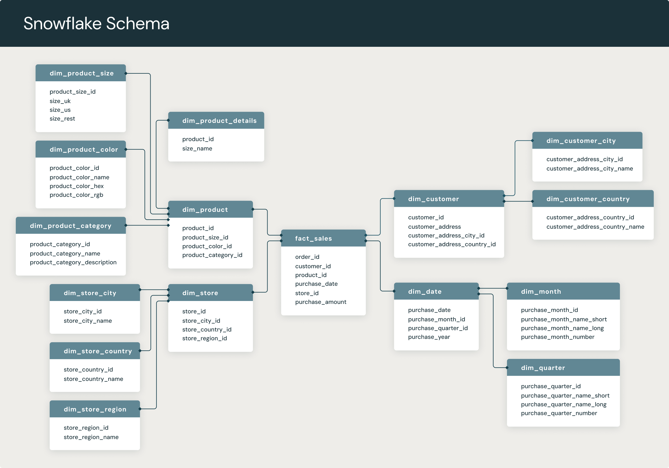
snowflake schema is a multi-dimensional data model that is an extension of a star schema, where dimension tables are broken down into subdimensions. Snowflake schemas are commonly used for business intelligence and reporting in OLAP data warehouses, data marts, and relational databases.

In a snowflake schema, engineers break down individual dimension tables into logical subdimensions. This makes the data model more complex, but it can be easier for analysts to work with, especially for certain data types.

It's called a snowflake schema because its entity-relationship diagram (ERD) looks like a snowflake, as seen below.

A snowflake schema diagram with a central fact table that connects to multiple dimensional tables and subdimensional tables via foreign keys.


Monday, June 10, 2024

Database Architecture


References: https://www.youtube.com/watch?v=9ToVk0Fgsz0

ETL Design Patterns

reference: https://www.youtube.com/watch?v=EmBwKA6vI14

Data Governance

Data governance is the system of internal policies that organizations use to manage, access, and secure enterprise data. While systems may vary in complexity from organization to organization, they always have some common features: internal processes, policies, defined roles, metrics, and compliance standards. The goal of the system is to help people efficiently and securely use the vast amounts of data generated by today’s enterprises.

Benefits:
  • Improved Data Management
  • Provide meaning and quality of data, Improved Data Quality
  • Regulatory, more consistent Compliance
  • Reduced costs and Increased Value.
  • Single source of Truth.
  • Establishing Data ownership & Accountability
Eg: Exchange datasets

Data Lineage

reference: https://www.youtube.com/watch?v=a4HPjtRHaHk

Data Modeling

What is an ER(Entity Relationship) Model?

An Entity Relationship Diagram is a diagram that represents relationships among entities in a database. It is commonly known as an ER Diagram. An ER Diagram in DBMS plays a crucial role in designing the database. Today’s business world previews all the requirements demanded by the users in the form of an ER Diagram. Later, it's forwarded to the database administrators to design the database.

Normalized Model?

Normalization is the method of arranging the data in the database efficiently. It involves constructing tables and setting up relationships between those tables according to some certain rules. The redundancy and inconsistent dependency can be removed using these rules in order to make it more flexible.

There are 6 defined normal forms: 1NF, 2NF, 3NF, BCNF, 4NF and 5NF. Normalization should eliminate the redundancy but not at the cost of integrity.

  1. Normalization is the technique of dividing the data into multiple tables to reduce data redundancy and inconsistency and to achieve data integrity. On the other hand, Denormalization is the technique of combining the data into a single table to make data retrieval faster.
  2. STAR Schema, Snowflake Schema comes into Picture in this case.

De-Normalized Model?

Deformalizing tables is basically creating a single source of truth when it comes to querying vast number of fact records that might have dimensional data spread across several tables. Having Facts and dimensions in a single table makes aggregations simpler, as the query runs faster.

Relational and Dimensional Models?

The relational model uses a collection of tables to represent both data and the relationships among those data.
Eg: Raw Layer


Dimensional Model:

Dimensional models are generally used for data warehousing scenarios, and are particularly useful where super-fast query results are required for computed numbers such as “quarterly sales by region” or “by salesperson”. Data is stored in the Dimensional model after pre-calculating these numbers, and updated as per some fixed schedule.

Eg: Curated Layer

What's the Difference Between a Data Warehouse, Data Lake, and Data Mart?

A data warehouse stores data in a structured format. It is a central repository of preprocessed data for analytics and business intelligence.

A data mart is a data warehouse that serves the needs of a specific business unit, like a company’s finance, marketing, or sales department. 

A data lake is a central repository for raw data and unstructured data. You can store data first and process it later on.


How to choose between star and snowflake schemas?

Generally speaking, a star schema is recommended if you have a few dimensions with low cardinality and limited levels of hierarchy. Additionally, if you need fast and simple queries with aggregated data and have ample storage space to tolerate some data redundancy, then this schema is ideal. On the other hand, a snowflake schema is best suited when you have many dimensions with high cardinality and multiple levels of hierarchy. This type of schema is also helpful when you need complex and detailed queries with granular data and want to avoid data inconsistency. Moreover, a hybrid approach that combines both schemas can be used depending on the specific data warehouse scenarios and trade-offs. For instance, a star schema can be used for simpler and more stable dimensions while a snowflake schema can be used for more complex and dynamic ones. Finally, you can also use a constellation schema that has multiple fact tables sharing some common dimension tables to support different business processes or analytical needs.


How to create a star schema?

A star schema is the Backbone of Dimensional Modeling. Below are the basic steps those I follow for this schema creation.

1. Understand and Select Business Process or Objective.
2. Define granular information to be stored in a table.
    Ideally, what should a row in the fact table need to represent?
    Eg: Daily trade value. etc
3. Identify Dimensions - like Calander, Location, Products etc
4. Identify Facts - measurable things like transactions, purchases etc
5. Build Star or Snowflake around a fact linking it with Dimensions. 


Data lake vs. Data warehouse


What is the difference between a data lake and a data warehouse?

A data lake and a data warehouse are two different approaches to managing and storing data. 

A data lake is an unstructured or semi-structured data repository that allows for the storage of vast amounts of raw data in its original format. Data lakes are designed to ingest and store all types of data — structured, semi-structured or unstructured — without any predefined schema. Data is often stored in its native format and is not cleansed, transformed or integrated, making it easier to store and access large amounts of data.

A data warehouse, on the other hand, is a structured repository that stores data from various sources in a well-organized manner, with the aim of providing a single source of truth for business intelligence and analytics. Data is cleansed, transformed and integrated into a schema that is optimized for querying and analysis.

Thursday, March 4, 2021

Spark Scala vs pySpark

Performance: Many articles say that "Spark Scala is 10 times faster than pySpark", but in reality and from Spark 2.x onwards this statement is no longer true. pySpark used to be buggy and poorly supported, but was updated well in recent times. However, for batch jobs where data magniture is more Spark Scala gives better performance.


Library Stack:

Pandas in Pyspark is an advantage.

Python's Visualization libraries complement pySpark. Where these are not available in Scala.

Python comes with some libraries that are well known for data analysis. Several Libraries are available like Machine learning and Natural Language Processing.


Learning python is believed to be easier than Scala.


Scala Supports powerful concurrency trough primitives like Akka's actors. Also has Future Execution context


Tuesday, March 2, 2021

Reconciliation in Spark

Input configuration as CSV and get primary keys for the respective tables and Updated_date

Source Unload - Select primarykeys, Updated_date from srcTbl1 where Updated_date between X and Y

Sink Unload - Select primarykeys, Updated_date from sinkTbl1 where Updated_date between X and Y


Recon Comparison Process:

Get Max Updated from srcTbl - val srcMaxUpdatedDate = srcDf.agg(max("Updated_date")).rdd(map(x => x.mkString).collect.toString


From Sink Table get only the columns whose Updated_date is less than Max Updated_date of Source.


val sinkDf = spark.sql("select * from sinkTbl where Updated_date <= ${srcMaxUpdatedDate}")


//This below function creates the SQL for comparision between source and sink tables and identifies if any of the records those were failed to get inserted to Sink table

keyCompare(spark,srcDf,sinkDf, primarykeys.toString.split(","))


def keyCompare(spark: SparkSession, srcDf: DataFrame, sinkDf: DataFrame, key: Array[String]): DataFrame = {

srcDf.createOrReplaceTempView("srcTbl")

sinkDf.createOrReplaceTempView("sinkTbl")

val keycomp = key.map(x => "trim(src." + x + ") = " + "trim(sink." + x + ")").mkString(" AND ")

val keyfilter = key.map(x => "sink." + x + "is NULL").mkString(" AND ")

val compareSQL = s" Select src.* from srcTbl src Left JOIN sinkTbl sink on $keycomp where $keyfilter"

println(compareSQL)

val keyDiffDf = spark.sql(compareSQL)

(keyDiffDf)

}

Sample Insert Compare would look like,

select src.* from srcTbl src left join sinkTbl sink on trim(src.PrimaryKEY1) = trim(sink.PrimaryKEY1) AND trim(src.PrimaryKEY2) = trim(PrimaryKEY2) where sink.PrimaryKEY1 is null and sink.PrimaryKEY2 is null


In the similar lines we can identify the records those were not updated during the delta process

select src.* from srcTbl src inner join sinkTbl sink on trim(src.PrimaryKEY1) = trim(sink.PrimaryKEY1) AND trim(src.PrimaryKEY2) = trim(PrimaryKEY2) where src.Updated_date != sink.Updated_date


def dateCompare(spark: SparkSession, srcDf: DataFrame, sinkDf: DataFrame, key: Array[String], deltaCol: String): DataFrame = {

srcDf.createOrReplaceTempView("srcTbl")

sinkDf.createOrReplaceTempView("sinkTbl")

val keycomp = key.map(x => "trim(src." + x + ") = " + "trim(sink." + x + ")").mkString(" AND ")

val compareSQL = s" Select src.* from srcTbl src Left JOIN sinkTbl sink on $keycomp where src.$deltaCol != sink.deltaCol"

println(compareSQL)

val keyDiffDf = spark.sql(compareSQL)

(keyDiffDf)

}

Wednesday, June 3, 2020

Handling Spark job Faliures

If we are doing bulky join and writing as Parquet, below is the screenshot of the failure Task.


Output - The estimated amount of records for this task after Join operation in Size and record count.
Shuffle Read - This can be considered as input for this job as it represents the mount of data involved or considered as input for this Join.

Shuffle Spill(Memory) - The amount of RAM consumed for this operation.
Shuffle Spill (Disk) - This indicates the amount of data written to Disk for this operation. Typically, this is not an ideal case to spill records to Disk and indicates that this stage is processing more data than it's capacity and have high chances of failure. While processing, as the data is more than the capacity of fit into RAM for that container, so it is written to Disk in compressed format.


Below is the ideal case:


Solution 1:

set spark.sql.shuffle.partitions

eg:

spark.conf.set("spark.sql.shuffle.partitions", 200)

The parameter that controls the parallelism during JOIN or Aggregrate operation that results from a shuffle is a parameter called spark.sql.shuffle.partitions. The reason why the default is 200 is from real-world experience that was found to be a very good default. But in practice, that value is usually always bad.

When dealing with small amounts of data, you should usually reduce the number of shuffle partitions otherwise you will end up with many partitions with small numbers of entries in each partition, which results in underutilization of all executors and increases the time it takes for data to be transferred over the network from the executor to the executor.

On the other hand, when you have too much data and too few partitions, it causes fewer tasks to be processed in executors, but it increases the load on each individual executor and often leads to memory errors. Also, if you increase the size of the partition larger than the available memory in the executor, you will get disk spills. Spills are the slowest thing you can probably be able to do. Essentially, during disk spills Spark operations place part of its RAM into a disk if it does not fit in memory, allowing Spark job to run well on any sized data. Even though it won't break your Pipeline it makes it super inefficient because of the additional overhead of disk I/O and increased garbage collection.

Therefore spark.sql.shuffle.partitions is one of the most frequently configured parameters when working with Spark.


Solution 2: Divide and conquer Approach

This is typically needed when the data being handled is more than the allocated Queue size. This is a case which I faced in one of my places those I worked, where I had to process and ingest huge sets of data but the Queue size allocated for my team is less than the data.
Not to worry in such cases we can divide the data into parts and then insert.

Eg: A case where we read data from 25 tables(either hive or RDBMS) , Join all these and write the result to MongoDB and consider the record count is 500 Million. Max memory limit per executor in the Queue is 15 GB and  this job fails at join phase.
So, divide the data to 10 equal parts and perform Joins on .5 Million records and ingest to MongoDB. Below are the steps to do this:

1. Create a temp table with only the primary keys and sort the keys in descending order.
2. Get Min and Max of the Primary keys and calculate the incrementaloffset by dividing it with the numParts which is 10 in this case.

Eg:
val numParts = 10
val incrementalOffSet = (maxPrimaryKeyVal - minPrimaryKeyValue)/numParts

Now incrementalOffSet  = ~.5M

3. Do a broadcast Join between this temp table of parted data with the main table. On doing this the main table's 0.5 Million records only will be involved in the transformation.

Reason of doing Broadcast Join is that the temp table will have only the primary keys and for millions of records it's size would be in MB's only and is safe to do it.

In case, if the primary key is not numeric(happens in case of hive tables), can pick any other Unique key or in the worst case create a Row_Number on the sorted records. All the need is to have a sorted set of dividable rows.

Below is the sample code and can be extended,


In this way, write a window and loop through the splitted data and complete the operation. This approach is helpful where the transformation logic cannot be splitted and data can be splitted.

Another approach where the number of tables being Joined can be splitted into parts.

Eg: In this case we have 25 tables. so perform 5 tables join each time.

Solution 3: 
RepartitionByRange

Consider a case where the data is Skewed which means if we have a record set of 10,000 records and is stored in 3 partitions and partition 1 has 7,000 records and the other 2 partitions has the remaining 3000 records. Or typically the data is not evenly distributed among the partitions.

To, distribute data evenly among all the partitions, use repartitionByRange API. This function takes 2 input parameters numberOf Partitions and ColumnName(s) on which the data has to be divided.

Eg: repartitionByRange ( 5, col("AccountId"))

for example, please refer https://www.waitingforcode.com/apache-spark-sql/range-partitioning-apache-spark-sql/read

Same can be achieved via bucketBy(), but repartitionByRange gives better results

Understanding DAG:


For the above Join operation where 20 tables data in Parquet is joined to form a single set. In Yarn UI, click on SQL in the pane. Below is the screenshot.


Level 1[Scan Parquet] - Indicates that the data is read from 3 parquet files as 3 tables

Level 2[Exchange] - As the data in HDFS or S3 is distributed among multiple nodes, Shuffle happens here and it is termed as Exchange.

Level 3[ Sort Merge Join] - In this stage Table 1 is Joined with Table 2 . And Table 2 is Joined with Table 3. Finally we will have 2 Datasets after this stage.


Going further, In the similar fashion all the tables would be joined.


Data Skewness :

https://selectfrom.dev/spark-performance-tuning-skewness-part-2-9f50c765a87e
https://www.youtube.com/watch?v=HIlfO1pGo0w